
Polynomial and Linear CART and their realization with R
Author: ZHANG Zihan The note is written in Markdown with PDF Version available.
Abstract
In this note, I would like to combine the regular decision tree model with linear regression and compare the results of both.
1. CART - Classification and regression tree
1.1 “Piecewise constant” (original) trees
“Cart” is an aggregate name of classification and regression tree, which is a statistical method for classification and regression that lies between parametric and non-parametric statistics. It provides a method of dividing the predictor space into various regions and do the fitness in each region. And usually it goes as piecewise constant form.
Here, the predictor space means the space that contains all the predictors, which could be denoted as \(\mathbf{x}=(x_1,x_2,…,x_n)\). Trees make fitness through generating leaves, meaning that each time the computer select one dimension (e.g. \(x_j\)) of the predictor space and split it and doing estimation in each part (\(x_j<c \ or \ x_j>c\) ).
Those trees can be used for both regression and classification with slight differences in their settings.
Suppose training data could be donated as \(D=\{(\mathbf{x_i} ,y_i)\}\) for \(N\) observations within the dataset and it have been separated into \(M\) regions, \(R_1,R_2,…,R_M\), by a tree. For each split region \(m\), the estimation is:
\[\overline{y_m}= \frac{1}{n_m}\sum_{x_i\in R_m}y_i\]and we can donate the regression function as:
\[\hat{f}(x)=\sum_{m=1}^M \overline{y_m}\cdot \mathcal{I}\{x\in R_m\}\]For classification trees, the setting in function slightly different with the counterpart of a regression trees. The estimation in each part could be represented as:
\[\widehat{p}_{j}^{m}=\frac{1}{n_{m}} \sum_{x_{i} \in R_{m}} \mathcal{I}\left\{y_{i}=j\right\}\]| where $$\widehat{p}_{j}^{m}=Pr(y=j | R_m)$$, which is the probability of each alternatives in each region. |
In each region, we choose the alternative with the highest probability within this region to be the prediction, which is:
\[c_{m}=\arg \max _{j} \widehat{p}_{j}^{m}\]And the classification function can be represented as:
\[\widehat{f}(x)=\sum_{m=1}^{M} c_{m} \cdot \mathcal{I}\left\{x \in R_{m}\right\}\]1.2 Polynomial (Linear) Trees
Usually, trees are commonly recognized as a method with as similar settings and outcomes as piecewise constant regression. Therefore, there would be some trees similar as piecewise linear or polynomial forms and we can substitute the function of original trees with a linear form to build a linear regression tree.
Suppose \(D=\{(\mathbf{x_i} ,y_i)\}\) comprises our training data. Similar as before, for each region \(R_j\in \{R_1,R_2,…,R_m\}\), we are able construct the regression in linear form:
\[\widehat{y_m}=\mathbf{\beta'x}\] \[\hat{f}(x)=\sum_{m=1}^M \widehat{y_m}\cdot \mathcal{I}\{x\in R_m\}\]For classification tree, we can apply the Logit regression instead of counting probability to make the classification.
\[\widehat{y_m}=F(\mathbf{\beta'x})\]where \(F(\beta'\mathbf{x})=\frac{1}{1+exp^{-1}(\beta'\mathbf{x})}\) and the regression is the same as the regression tree.
\[\hat{f}(x)=\sum_{m=1}^M \widehat{y_m}\cdot \mathcal{I}\{x\in R_m\}\]1.3 Error Term
In the process of construction of trees, we usually minimize the in sample error within each region and then sum them together, which means that
\[\mathrm{RSS}=\sum_{m=1}^{M} \sum_{x_{i} \in R_{m}}\left(y_{i}-\widehat{y}_{m}\right)^{2}\]However, due to the goal of minimizing RSS for the whole region, it is reasonable to project that a couple of leaves would be generated to minimize the in sample error. As a result, the tree might be too large to predict because of potential overfitting problems. Hence, we apply “Pruning” method, including the penalty term for tree’s number of leaves to preventing from generating too many branches and potential overfitting problems.
\[Error=\sum_{m=1}^{|T|} \sum_{x_{i} \in R_{m}}\left(y_{i}-\overline{y}_{m}\right)^{2}+\alpha|T|\]where \(T\) is the size of trees and \(\alpha\) is a tuning parameter that controls the magnitude of penalties for magnitude of a tree.
2. Realization of linear trees in R
The instructor provided methods of realizing regular trees (piecewise constant) in class, here I would attempt to explore a method to build linear trees in R.
Firstly, I would like to generate some data for the simulation. In order to get a better visualization, I generated with only two dimensions (\(x_1\)and\(x_2\)) for regression and \(y_i=2 -(x_{1i}^2+x_{2_i}^2+\epsilon_i)\)
for (i in 1:2) {
x1 <- runif(500,min = -1,max = 1)
x2 <- runif(500,min = -1,max = 1)
y <- -x1^2-x2^2+2+rnorm(500,mean = 0,sd = 0.02)
if(i==1)
  trset <- data.frame(y,x1,x2)
else
  teset <- data.frame(y,x1,x2)
}
2.1 Original Tree Models
Decision trees follow the ideas of separating the entire space into various regions to gain more precise estimation for the original data space. Here, we can build a tree to fit the data generated previously.
From the figure, it is evident that a tree with 12 leaves minimize the out sample error.

Therefore, the tree is as follows.

# Trees
library(rpart)
library(rpart.plot)
set.seed(123)
fit.tree = rpart(y~x1+x2,trset,model = F,control=rpart.control(cp=0))
printcp(fit.tree)
plotcp(fit.tree)
fit.tree= prune(fit.tree,
            cp=fit.tree$cptable[which.min(fit.tree$cptable[,"xerror"]),"CP"])
rpart.plot(fit.tree,type = 2)
y.treehat <- predict(fit.tree,teset)

fit.tree.error <- sum((y.treehat-teset$y)^2)/500
fit.tree.error
# [1] 0.3102634
The out sample error is approximately 0.31 for tree model.
2.2 Piecewise Polynomial (Linear) Regression for higher dimensions
In “regression” section, we have talked about the piecewise method for regression, which provided an advanced approach for better precision in local areas. With the similar motivation with trees, we could apply the piecewise regression for multiple dimensions and variables, seeking for the better accuracy in the divided regions.
For example, I apply piecewise method for the previous data, setting knots at 0.5, 0 and -0.5 for both \(x_1\) and \(x_2\) and divided the whole plain into 16 parts. We can see the characteristics of data from the following diagram.
# Piecewise linear model
library(splines)
library(AER)

fit1 <- lm(y ~ bs(x1,knots = c(-0.5,0,0.5),degree = 1)+bs(x2,knots = c(-0.5,0,0.5),degree = 1),data = trset)

y.hat <- predict(fit1,teset)
fit.hat.error <- sum((y.hat-teset$y)^2)/500
fit.hat.error
# [1] 0.001103903
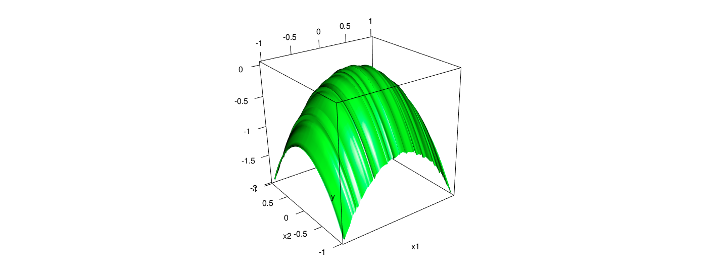

The fitted plain and data points with piecewise linear model for the data is as follows.
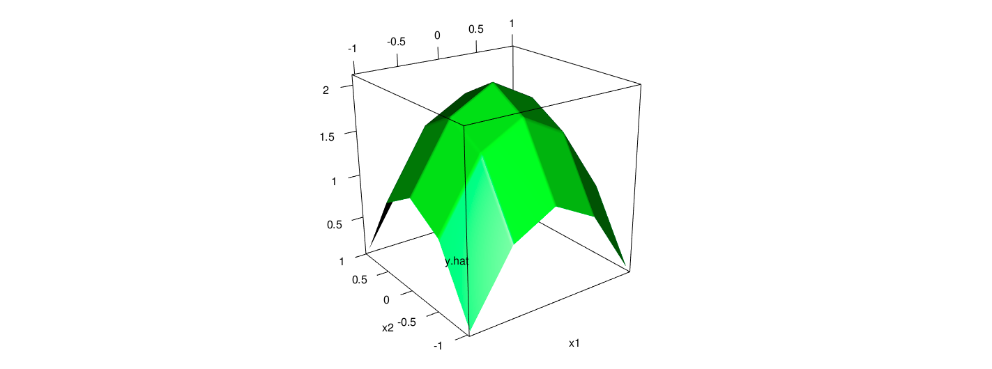

As the computation, the out of sample error is 0.0011, indicating the estimation with piecewise method is pretty good. Intuitively, from the two scatter plots, it is obvious that the results from the piecewise method is quite close to their actual values. Furthermore, the fitted error is considerably smaller than the counterparts of previous tree model.
2.3 Combination of Trees and Piecewise Polynomial Method
The mechanism of piecewise polynomial or linear tree is simple because we can simply substitute the regression function from mean function to linear or polynomial functions. The most pure procedure with the same idea of trees is that generating leaves first and pruning afterwards. However, due to the limitation of my programing skill, I did not find any programs that could make the idea into realization. Thus, I suppose it could be a wise idea of using knots of original trees as the separation boundary, especially for regression trees. The underlying consideration is that notwithstanding taking average could not be the best approach for regression tree, it could be helpful to settle the boundary of sub-spaces with the idea of minimizing the out sample error. Within these separated regions, models with higher complexity could be applied for better estimation.
# combination
library(dplyr)
leaf1 <- subset(trset,(x1 < -0.83)&(x2< - 0.62))
leaf2 <- subset(trset,(x1 < -0.83)&(x2>= 0.69))
leaf3 <- subset(trset,(x1 < -0.83)&(x2< 0.69)&(x2>= - 0.62))
leaf4 <- subset(trset,(x1 >= 0.91))
leaf5 <- subset(trset,(x1 < 0.91)&(x1>= 0.56)&(x2< -0.65))
leaf6 <- subset(trset,(x1 < 0.91)&(x1>= 0.56)&(x2>= 0.54))
leaf7 <- subset(trset,(x1 < 0.91)&(x1>= 0.56)&(x2< 0.54)&(x2>= -0.65))
leaf8 <- subset(trset,(x1 >= -0.83)&(x1< 0.56)&(x2< -0.82))
leaf9 <- subset(trset,(x1 >= -0.83)&(x1< 0.56)&(x2>= 0.57)&(x1< -0.38))
leaf10 <- subset(trset,(x1 >= -0.83)&(x1< 0.56)&(x2>= 0.57)&(x1>= -0.38))
leaf11 <- subset(trset,(x1 >= -0.83)&(x1< 0.56)&(x2>= -0.82)&(x2< -0.49))
leaf12 <- subset(trset,(x1 >= -0.83)&(x1<= -0.56)&(x2>= -0.49))
leaf13 <- subset(trset,(x1 >= 0.31)&(x1<0.56)&(x2>= 0.097)&(x2< 0.57))
leaf14 <- subset(trset,(x1 >= 0.31)&(x1<0.56)&(x2>= -0.49)&(x2< 0.097))
leaf15 <- subset(trset,(x1 >= -0.56)&(x1<0.31)&(x2>= 0.49)&(x2< 0.57))

fitc1 <- lm(y~x1+x2,data = leaf1)
fitc2 <- lm(y~x1+x2,data = leaf2)
fitc3 <- lm(y~x1+x2,data = leaf3)
fitc4 <- lm(y~x1+x2,data = leaf4)
fitc5 <- lm(y~x1+x2,data = leaf5)
fitc6 <- lm(y~x1+x2,data = leaf6)
fitc7 <- lm(y~x1+x2,data = leaf7)
fitc8 <- lm(y~x1+x2,data = leaf8)
fitc9 <- lm(y~x1+x2,data = leaf9)
fitc10 <- lm(y~x1+x2,data = leaf10)
fitc11 <- lm(y~x1+x2,data = leaf11)
fitc12 <- lm(y~x1+x2,data = leaf12)
fitc13 <- lm(y~x1+x2,data = leaf13)
fitc14 <- lm(y~x1+x2,data = leaf14)
fitc15 <- lm(y~x1+x2,data = leaf15)

leaf1 <- subset(teset,(x1 < -0.83)&(x2< - 0.62))
leaf2 <- subset(teset,(x1 < -0.83)&(x2>= 0.69))
leaf3 <- subset(teset,(x1 < -0.83)&(x2< 0.69)&(x2>= - 0.62))
leaf4 <- subset(teset,(x1 >= 0.91))
leaf5 <- subset(teset,(x1 < 0.91)&(x1>= 0.56)&(x2< -0.65))
leaf6 <- subset(teset,(x1 < 0.91)&(x1>= 0.56)&(x2>= 0.54))
leaf7 <- subset(teset,(x1 < 0.91)&(x1>= 0.56)&(x2< 0.54)&(x2>= -0.65))
leaf8 <- subset(teset,(x1 >= -0.83)&(x1< 0.56)&(x2< -0.82))
leaf9 <- subset(teset,(x1 >= -0.83)&(x1< 0.56)&(x2>= 0.57)&(x1< -0.38))
leaf10 <- subset(teset,(x1 >= -0.83)&(x1< 0.56)&(x2>= 0.57)&(x1>= -0.38))
leaf11 <- subset(teset,(x1 >= -0.83)&(x1< 0.56)&(x2>= -0.82)&(x2< -0.49))
leaf12 <- subset(teset,(x1 >= -0.83)&(x1<= -0.56)&(x2>= -0.49))
leaf13 <- subset(teset,(x1 >= 0.31)&(x1<0.56)&(x2>= 0.097)&(x2< 0.57))
leaf14 <- subset(teset,(x1 >= 0.31)&(x1<0.56)&(x2>= -0.49)&(x2< 0.097))
leaf15 <- subset(teset,(x1 >= -0.56)&(x1<0.31)&(x2>= 0.49)&(x2< 0.57))

y.hat.c1 <- predict(fitc1)
y.hat.c2 <- predict(fitc2)
y.hat.c3 <- predict(fitc3)
y.hat.c4 <- predict(fitc4)
y.hat.c5 <- predict(fitc5)
y.hat.c6 <- predict(fitc6)
y.hat.c7 <- predict(fitc7)
y.hat.c8 <- predict(fitc8)
y.hat.c9 <- predict(fitc9)
y.hat.c10 <- predict(fitc10)
y.hat.c11 <- predict(fitc11)
y.hat.c12 <- predict(fitc12)
y.hat.c13 <- predict(fitc13)
y.hat.c14 <- predict(fitc14)
y.hat.c15 <- predict(fitc15)

fit.c.error <- (sum(y.hat.c1-leaf1$y)+sum(y.hat.c2-leaf2$y)+sum(y.hat.c3-leaf3$y)+sum(y.hat.c4-leaf4$y)+sum(y.hat.c5-leaf5$y)+
                     sum(y.hat.c6-leaf6$y)+sum(y.hat.c7-leaf7$y)+sum(y.hat.c8-leaf8$y)+sum(y.hat.c9-leaf9$y)+sum(y.hat.c10-leaf10$y)+
                     sum(y.hat.c11-leaf11$y)+sum(y.hat.c12-leaf12$y)+sum(y.hat.c13-leaf13$y)+sum(y.hat.c14-leaf14$y)+
                     sum(y.hat.c15-leaf15$y))^2/500
fit.c.error
# 0.005494581
From the result, we can see that the piecewise linear tree model also reduced the sample error significantly compared to the tree model.
Reference
[1] Eberly College of Science, Penn State University, Piecewise linear regression models, STAT 501, https://newonlinecourses.science.psu.edu/stat501/node/310/
[2] Chaudhuri P , Huang M C , Loh W Y , et al. Piecewise-Polynomial Regression Trees[J]. Statistica Sinica, 1994, 4(1):143-167.
[3] Quinlan J R . Simplifying Decision Trees[J]. International Journal of Human-Computer Studies, 1987, 27(3):221-234.
[4] Hadley Wickham, ggplot2:数据分析与图形艺术[M], 西安交通大学出版社, 2013
[5] Jiaming Mao, Regression, https://jiamingmao.github.io/data-analysis/assets/Lectures/Regression.pdf
[6] Jiaming Mao, Decision Tree and Ensemble Method, https://jiamingmao.github.io/data-analysis/assets/Lectures/Decision_Trees_and_Ensemble_Methods.pdf