The Bootstrap Estimate for Standard Error

Author: Zihan Zhang

Abstract

Bootstrap is a simple method used to estimate the standard error of an unknown population with only a sample. In this note, I would like to write an brief introduction about the Bootstrap as well as its realization with some other softwares except for R.

1. Nonparametric Bootstrap

1.1 Methodology

Bootstrap, firstly introduced in 1979, provides a relatively simple way to calculate the standard error of the estimator just based on the sample we known. Actually, Bootstrap that we have discussed in class is the non-parametric one, which means it does not be involved in any theoretical derivations. It enjoys the advantages of being being able to finish the whole process by computers themselves.

Suppose we have an underlying population \(F\) with a coefficient \(\theta\) describing its feature and both of them are unknown. Also, we have a sample \(\mathbf{x} = (x_1,x_2,...,x_n)\) comprising some individuals (\(x_i\)) generated from \(F\). In statistics, we are able to estimate \(\theta\) with the estimator \(\hat{\theta}=s(\mathbf{x})\) through some derivations. The Bootstrap was introduced to measure the accuracy of \(\hat{\theta}\).

From the known sample, we are able to generate the Bootstrap sample, which is defined to be a random sample of size n with replacement from the known sample \(\mathbf{x}\). It could be donated as \(\mathbf{x}^*=(x_1^*,x_2^*,...,x_n^*)\), where the star notation manifest the \(\mathbf{x^*}\) is not the actual set of \(\mathbf{x}\), but rather a randomized and replaced version of initial sample \(\mathbf{x}\).

Next, we would like to evaluate the Bootstrap replication corresponding to each Bootstrap sample and calculate the \(\hat{\theta(i)}=s(\mathbf{x}^{*i})\) for each Bootstrap sample. Having those done, we are able to estimate the stand error by the sample standard deviation of N replications. The equation is as follows.

where \(\theta^*(\bullet)=\frac{1}{N} \sum_{i=1}^N \theta^*(i)\).

1.2 Merits and demerits

One of the merits of Bootstrap is its simplicity, which makes it possible to extend the sample size in a direct method. Therefore, if the sample describes the population very well, then it is straightforward to compute the standard error without models and assumptions. Besides, Bootstrap provides an appropriate way to check the stability of the result.

On the other hand, if the sample could not be a represent of the underlying population, it is true that the result with Bootstrap is not much reliable.

2. Parametric Bootstrap

The parametric Bootstrap for estimating standard error shares the same ideas of the non-parametric one, which is generating Bootstrap samples with limited information.

The only difference between those two is parametric Bootstrap method assumes that the form of underlying population \(F\) is known. In other words, we can assume that the sample comes from a particular distribution and it is possible to estimate the coefficients (\(\theta\)) of the distribution based on the sample. Therefore, with the estimated coefficients (\(\hat{\theta}\)) as well as the population (\(\hat{F}\)), we are able to use the parametric Bootstrap, but with a different manner as before. Here, instead of sampling with replacement from the known data, we draw N samples from the parametric estimation of underlying population \(\hat{F}\), which could be shown as \(\hat{F} \rightarrow (x_1^*,x_2^*,...,x_n^*)\).

Having drawn the Bootstrap samples, the left procedures for estimating \(\widehat{SE_N}\) are the same as those of non-parametric Bootstraps.

3. Translate the code into MATLAB language

The instructor provides a method of realization of the Bootstrap in R, here I would like to make it available in MATLAB.

The program could be written in function, which is as follows.

function main_bootstrap()
%% import the data from R, "Portfolio" is the same dataset from R.
Portfolio=xlsread('Portfolio.xlsx')

%% generate one bootstrap sample and calculate the alpha.
index=randint(1,length(Portfolio),[1 length(Portfolio)]);
alpha = return_alpha(Portfolio,index) 

%% do bootstrap manually.
A=[]
B=1000
for i=1:B
A(i)=return_alpha(Portfolio,randint(1,length(Portfolio),[1 length(Portfolio)]));
end

mu = mean(A)
sd = std(A)

%% This is the function used for computing alpha.
    function alpha= return_alpha(data,index)
        x=data(index,1);
        y=data(index,2);
        c=cov(x,y)
        alpha=((var(y)-c(1,2))/(var(x)+var(y)-2*c(1,2)))
    end
end

Also, we can realize it without matlab functions.

clear
Portfolio=xlsread('Portfolio.xlsx')
index=randint(1,length(Portfolio),[1 length(Portfolio)]);

A=[]
B=1000
for i=1:B
    index=randint(1,length(Portfolio),[1 length(Portfolio)]);
    x=data(index,1);
    y=data(index,2);
    c=cov(x,y)
    alpha=((var(y)-c(1,2))/(var(x)+var(y)-2*c(1,2)))
    A(i)=alpha;
end

mu = mean(A)
sd = std(A)

Having finished the process, I would like to compare the results from both softwares.

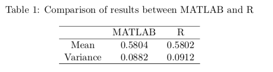
It is evident that the results from two softwares are similar.

Reference

[1] Efron B., Tibshirani R. (1993).An introduction to Bootstrap, ISBN 0-412-04231-2.

[2] Bootstrapping (statistics), https://en.wikipedia.org/wiki/Bootstrapping_(statistics).

[3] Jiaming Mao, Regression, https://jiamingmao.github.io/data-analysis/assets/Lectures/Regression.pdf

Applendix

This notes is also written in \(\mathbf{LaTex}\) with PDF Version available.

Code and data are available here